
17 May 2024 19:00 UTC

| Age: | 9.651 |
| Constellation: | Leo |
| Phase: | 71.29° |
| Diameter: | 29.52' |
| Distance: | 404675 km |
| Right ascension: | 11.5685h |
| Declination: | 4.9609° |
| Sub-solar longitude: | 65.555° |
| Sub-solar latitude: | 1.07° |
| Sub-Earth longitude: | 0.844° |
| Sub-Earth latitude: | -2.556° |
| Position Angle: | 21.834° |
Lunar Photography
Once you took a photo of the Moon you are done. Nope, because of the lunar phases changing illumination angles from either east or west cast various shadows giving surface regions a different face every time. Achievable image quality strongly depends on atmospheric condition in that you can almost always improve over your previous images at a later date. As an Apollo astronaut once marvelled, "It's a bleak beauty".
Though the moon exhibits subtle colors, in particular the northern regions, many astro-photographers prefer to use monochrome cameras in conjunction with an IR-pass filter in order to obtain higher resolution and sharpness benefitting from the high near-infrared response of modern astro-cameras.
The Moon is about a quarter the diameter of Earth but exhibits extreme natural and geological dimensions. Some peaks of the rugged mountain chain Montes Apenninus rise as high as 5 kilometers (3 miles) casting long shadows. Crater Copernicus is 3.8 kilometers (2.36 miles) deep as are many more, wide or small. Rupes Altai is an escarpment located south of Mare Nectaris stretching over 420 kilometers (260 miles). Most craters contain a dozen or more craterlets and have central peaks casting shadows. Under the right illumination and timing stunning pictures of such features are possible -- the exciting side of lunar photography.
Thanks to the moon's libration (wobbling effect), 59% of its surface is observable from Earth. The maximum libration angle is: 1.54° (equator to ecliptic inclination) + 5.15° (ecliptic to orbital plane inclination) = 6.69°. Libration occurs in both lunar latitude and longitude and at times brings far side features or parts of them into view, such as the entire Mare Humboldtianum at the northeastern edge above the better known Mare Crisium.
Since the lunar orbit around Earth is of elliptical shape its distance to Earth changes strictly speaking every second (orbital speed = 1.022km/sec). When reaching its closest orbit location the distance is around 362,600 kilometers (225,310 miles) while the farest point is at around 405,400 kilometers (251,903 miles), after all a difference of 42,800 kilometers (26,595 miles), or over 12 times the lunar diameter. Consequently, when nearest, the Moon is apparently larger therefore better positioned for imaging, however, we may be splitting hairs since seeing is the more dominant factor influencing the resolution and quality of our images.
 Mare Humboldtianum (in infrared) at favorable libration in longitude. Mars of the same evening on October 2nd., 2020 is inserted to scale.
Equipment
Telescope
In the interest of good resolution, a telescope with at least 5-inches (127mm) aperture, Newtonian or Cassegrain, will be fine. A Newtonian is most affordable and the 'fast' with typically F5 focal ratio sufficing with short exposure times, but is quite heavy therefore requiring a sturdy mount. More costly than Newtonians, Cassegrains come with a focal ratio of F10 and with a long native focal length. A variation, the Maktsutov Cassegrain, has a slower focal ratio of around F12 to F15 and is said to produce sharp images. Cassegrains have a shorter tube and weigh less than comparable Newtonians. Owing to its design, the aperture of reflectors is obstructed by a secondary mirror. Consequently, a 6-inch scope is a little over true 5 inches. If you choose an 8-inch scope you will get true 6.5 to 7 inches depending on the size of the secondary mirror.

Please be aware that large telescopes do not only collect more light but also way more air turbulences as compared with smaller telescopes. With 10 and more inches aperture you depend a lot on good seeing, but when seeing is really good the images will knock you out. Telescopes from 5 to 8 inches, too, can produce remarkable images. Refractors can as well be used but are quite expensive with growing aperture. So-called "field flatteners" (for refractors) and "coma correctors" (for Newtonians) are not essential because the sensor of a 'planetary' camera is rather small. Besides some budget, choosing a telescope requires a great deal of diplomacy and compromising.
Tracking Mount
The most important gear is an electronic equatorial mount capable of accurate tracking. The heavier the telescope the sturdier a mount is required. High magnifications typically required for lunar imaging call for accurate tracking. The mount should be specified for a payload of, say, 1.3 times the weight of your complete imaging gear. Autoguiding is not necessary.
Camera
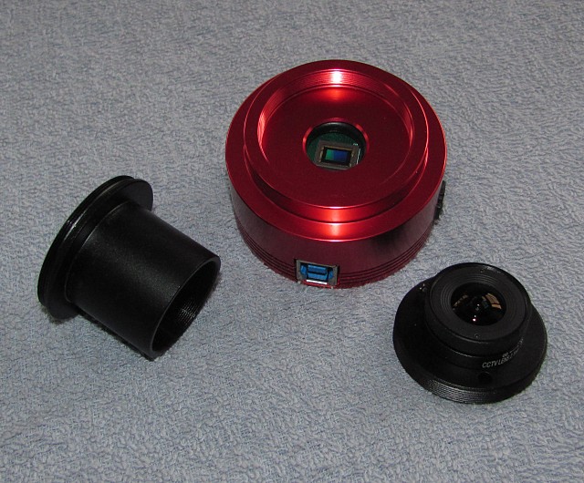
A "planetary" CMOS astro-camera records uncompressed videos containing thousands of frames from which a certain percentage (typically the best 10% to 20%) are used for stacking. Available in color and monochrome, planetary cameras sport sensors up to full HD resolution (1920 x 1080 pixels), resulting in a narrow field of view which is desirable for imaging the Moon and the planets. Color cameras make it easy to image painlessly within short time. Monochrome cameras offer higher resolution and sharpness. In order to produce a color image with a monochrome camera a set of color filters is required significantly extending imaging and post-processing time. A filter set including wheel costs about the same as a color camera in that ownership of both a color and a monochrome camera is most efficient. Cameras containing the Sony IMX290/462 sensor are ideal for our purpose.
Filters

Two types of filters are essentially required because a CMOS camera is sensitive to both visual and near infrared wavelengths. If used without filters images will look notably smeared with pastel colors. An infrared cut filter passes visual light only. It is indispensible for color photography. An infrared pass filter blocks visual light and can be used with both color and monochrome cameras while images are usually converted to gray scale because infrared is colorless. When the atmosphere is turbulent, an IR-pass filter can help reduce the effect of blurring. IR-pass filters are available with kick-off wavelengths between about 600nm and 850nm. With increasing wavelength the camera's response drops in that filters with long wavelengths require longer exposure times. CMOS cameras containing the Sony IMX462 sensor are highly sensitive to infrared, therefore hardly compromising exposure time when using IR-pass filters up to 750nm. When frequently imaging in both wavelength domains, a (mechanical) filter wheel can help reduce adrenaline flow.
Computer
Consider a laptop with SSD disk and powered USB-3.x port since mechanical hard disks are often too slow resulting in intermediate buffering of frames in memory, then saving the buffered frames to hard disk, a process which can significantly extend the time needed for writing a video file. Since you will be saving several Gigabytes per video file (ex.: 6000 frames, 8-bit depth = 12GB) the capacity of the hard disk should be generous, at least, say, 512 Gigabytes.
Software
- Capture: Please look for SharpCap or FireCapture or applications offered by camera manufacturers.
- Stacking: Please look for Autostakkert!3 which is the optimal choice though many prefer Registax6.
- Post-processing: GIMP, Photoshop or similar image processing applications.
- Mosaics: For image stitching, among other choices, MS-ICE is an accurate, simple-to-use application.
Other
Do not forget to prepare a table and a chair plus a power supply for both the laptop (and the tracking mount). An LED light will help avoid hitting the wrong keyboard keys. Outside there is no roof to hit or go through.
Example Gear
There is much more out there though...
If you cannot rule out giving up the hobby sooner or later, a low-cost entry equipment may be a reasonable start. A lot of people use a Sky-Watcher Mak127 (5-inch) on a AZ-GTi altaz mount (sold bundled) with a ZWO ASI224MC or QHY224C color camera. It is a low end camera but its sensitivity and image quality are everything else but low. The Mak127 is also great for visual observations in case your kids take over.
Provided you intend to enjoy the hobby for a long time you may consider an 8-inch Cassegrain on a solid mount with a ZWO ASI290MM/MC or QHY290M/C camera. Assuming affordability and endless motivation, go for a 11 or 14-inch Cassegrain telescope (plus a 6-inch Newtonian for times when seeing is bad and the night still long).
Affordable equatorial mounts are offered by manufacturers such as Sky-Watcher, Celestron and Orion. Make sure the mount can handle the weight of the telescope plus imaging gear.
Whether you choose a Cassegrain or a Newtonian, you may wish to increase the focal length (magnification) using a 2x or 3x barlow lens of high quality since the barlow is often the weakest element in an optical train. Too much magnification is not recommended.

Since the camera's infrared response is usually lower than its response to visual light (vice-versa for the IMX462 sensor) the IR-pass filter cut-off wavelength should not be too long. Small aperture telescopes are less prone to air turbulences in that about 640nm are sufficient. For larger telescopes, say, 10 inches and more, 740nm will be more suitable. Filters are usually not parfocal, meaning that the telescope needs to be refocused when swapping filters.
Lunar imaging does not require a high-end laptop. With its fast SSD and USB, the Thinkpad E590 laptop, for instance, is ideal for video capture, but not water-proof, so, place your double-star drink away from the laptop.
Budget
Estimated cost...
An independent choice of intermediate-level equipment (new) with focus on best economy would suggest a total cost of about 2,200 USD. It is merely a rough guideline, your financial mileage and preferences may vary. You may also wish to consider used gear.
| Mount | Orion Sirius EQ-G (13kg payload) | 1100 USD |
| Telescope | Sky-Watcher 200PDS (8-inch Newtonian, F5, 200/1000mm) | 425 USD |
| Camera | ZWO290MM/QHY5III290M (1936×1096/1920x1080 pixels monochrome) | 450 USD |
| Other | Barlow (2x/3x), filters | 150 USD |
Here a calculation for portable beginner-level equipment amounting to about 1,100 USD:
| Mount/Telescope | Sky-Watcher Mak127 (5-inch Maktsutov, F12, 127/1500mm) on AZ-GTi mount (5kg payload) | 650 USD |
| Camera | ZWO224MC/QHY5III224C (1304×976 pixels color) | 280 USD |
| Other | Barlow (2x/3x), filters | 150 USD |
Objectives
The key points...
The aim is to produce videos at shortest possible exposure time and fast frame rate in particular when seeing is poor and persistently rolling in clouds are disturbing. Equally important is low noise. Noise can be reduced by choosing the lowest feasable gain and a large number of frames to stack. Naturally, imaging the Moon at good seeing is the best guarantor of success.
Infrared pass filters compensate a lot for poor seeing but need longer exposure times as the camera's infrared response is lower than its color response. In case of the ASI290MM, the exposure time with an IR640nm pass filter is about half that of an IR740nm filter -- a significant benefit when seeing is not too bad.
Quality IR-cut filters pass more than 95% of the light hence hardly sacrificing exposure time. It is a dance on a rope. Either you record in visual light resulting in the shortest possible exposure times and fastest frame rates, or in infrared with longer exposures and slower frame rates, but less prone to poor seeing. When your time and clouds allow, image in both domains and select the keepers after post-processing.
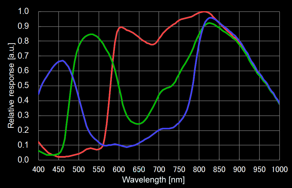
ASI462MC/QHY5III462C
Response of the ASI462MC/QHY5III462C color cameras. The response in near infrared is higher than in color, a unique characteristic which helps reduce exposure times for infrared imaging.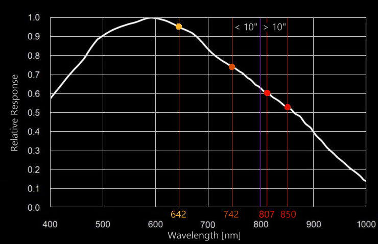
ASI290MM/QHY5III290M
Response of the ASI290MM/QHY5III290M monochrome cameras. The response in near infrared drops past 600nm and is around 50% at 850nm. However, the response is still high with typical IR-pass filters of 640 to 740nm.The curves should be taken with a grain of salt as for most cameras the accurate relative response, also specified as quantum efficiency, QE, is unconfirmed.
News just in: In November 2020, QHYCCD has launched its QHY5III485C, an 8.3 megapixels 4K color camera with 3840×2160 pixels coring the 7.2 x 4.5mm dimensioned Sony IMX485 sensor. It is basically QHY's QHY5III290C but with four times the chip area resulting in twice the field of view. In 2x2 binning mode the cell size doubles to 5.8µm while still providing HD resolution.
Test with ASI290MM...
With Baader UV/IR-Cut Filter

Exposure 2ms, gain 200, 170fps
With Sightron IR640nm Pass Filter

Exposure 4ms, gain 200, 170fps
With Astronomik IR742nm Pass Filter

Exposure 8ms, gain 200, 120fps
This equally stacked and processed monochrome image trio compares the results with various filters under turbulent air. Test equipment: ASI290MM camera set to mono-8 and 10-bit ADC, Ø150mm f5 Newtonian with 2x barlow (FL=1500mm, f10). Obviously, the differences are subtle. Short exposure times freeze the frames while infrared is less prone to seeing. The IR640nm pass filter allows short exposure times while contributing the infrared advantage. Click on an image to view its full size.
Capture Parameters
About color spaces and frame rates...
Color Spaces
The keys to brilliant images next to good seeing are short exposure time and a consequently fast frame rate (fps). The shorter the exposure the faster the achievable frame rate. The frame rate depends on various factors.
- Monochrome cameras provide 8-bit or 16-bit Mono 'color spaces' where 8-bit yields the faster frame rate, about twice as fast as 16-bit. Color cameras provide '8-bit and 16-bit Raw', 'RGB24', and '8-bit Mono'. 8-bit Raw yields twice the frame rate of 8-bit Mono.
- The camera can use either a 10-bit ADC (high speed mode ON) or 12-bit ADC (high speed mode OFF). The 10-bit ADC provides 1024 brightness levels (faster frame rate) while the 12-bit ADC provides 4096 levels hence the better contrast and detail but at about half that of the 10-bit frame rate. There is hardly any difference in frame rate when the exposure time exceeds 10ms (as found with an ASI290MM). For the moon and planets 8-bit depth with 10-bit ADC is basically sufficient, but note that the 12-bit ADC can help reduce read noise and increase contrast.
- Reduction of the image size (ROI = Region of Interest) too results in faster frame rates. While for the Moon the maximum size is desirable, planets do not require that much space. Often an ROI of 320 x 240 pixels is quite sufficient for planets. IMX290 sensor based cameras sport a frame rate of 170fps at maximum ROI and can exceed 300fps with 640 x 480 pixels or 700fps with 320 x 240 pixels through the camera's 10-bit ADC.
NOTE: 16-bit mono and 16-bit Raw provide 65,536 brightness values, however, the camera's 12-bit ADC outputs 4,096 maximum. Therefore, 16-bit color spaces can safely be ignored.
File Formats
Select the most robust...
All cameras can save videos as *.AVI or *.SER. While AVI can be played on numerous applications, SER is more robust and less error-prone as specifically concepted for astronomy image capture. The choice of SER is recommended and fully compatible with the Autostakkert!3 stacking software.
The document file of SharpCap explains further details.
Post Processing
In Photoshop...
There are certainly more professional procedures while the quality of unprocessed images vary. The following table contains the basic steps employed by the author. Please remember, "less is more".
Hint: Purposely under-expose the SER video a little bit to avoid saturation during processing. Then, in Photoshop,
| Menu Item | Image | Description |
| Image/Adjustment/Curves |  |
Raise the Curve, crop away stacking artefacts and duplicate the layer. |
| Filter/Other/High Pass |  |
Apply high pass filter (100%) and blend the layers with Soft Light. This adds sharpness, contrast and lets the image look deeper. You can adjust the opacity of the layer if need be. Next, select Layer/Flatten Image. |
| Filter/Blur/Gaussian Blur |  |
Apply a Gaussian Blur (Radius 0.5 pixels) to smooth noise. |
| Filter/Sharpen/Unsharp Mask |  |
If not sharp enough apply a light Unsharp Mask (radius 2-5 pixels), and another Gaussian Blur (do not overdo sharpen). |
| Filter/Noise/Reduce Noise |  |
In case of a color image (not for monochrome), apply Noise Reduction and disable all adjustments except Color Noise Reduction. |
| Image/Adjustments/'Hue/Saturation' |  |
If you wish to create a mineral moon, increase Saturation in several small steps of say 20 or 30 each until colors emerge to your liking. |
| Image/Mode |  |
Autostakkert!3 saves file in RGB color 16-bit format. Reduce to 8-Bits/Channel when the SER video is in 8-bit. Select Grayscale if you are processing monochrome or infrared images. This will significantly reduce file size. |
Hints
This is not new to most of you. Anyway:
- Set up the gear and be sure to achieve best polar alignment, thus tracking accuracy.
- Image under clear, steady atmospheric condition and wind-protected.
- Wait for the maximum elevation of the Moon near meridian transit, 45° and higher would be great (location and season dependent).
- Image in infrared and/or with shortest possible exposure time at maximum frame rate when seeing is unfavorable.
- In the capture software, select 8-bit color spaces (raw-8 for color or mono-8 for monochrome).
- In the capture software, select "High Speed Mode" (10-bit ADC), unless the image looks noisy.
- Slightly under-expose the video (can be compensated for during processing).
- Make sure to get pin-point focus (magnify the preview 125-150% to confirm).
- Record the video with a computer equipped with an USB3.x port and a SSD disk.
- Try first with a 6000 frames video and stack 10% in Autostakkert!3 with pre-sharpen.
 ⛶ Full Screen
Lots of tutorials about Autostakkert!3 can be found online while the application provides a Help section. The key here is "Sharpened, Blend Raw in for..." (at the right of the right window).
The sharpen function of Autostakkert!3 is awesome. The lower the set percentage the stronger the sharpen effect. When imaging at native 750mm focal length and drizzle 1.5x then 50% is just right, while 20% are fine for FL=1500mm and 15% for FL=2250mm. This is based on the author's Ø150mm Newtonian and may vary for other telescopes (and seeing conditions). The strength of sharpening also varies whether you drizzle or not. The effect is stronger without drizzle. A few tests are recommended to find the optimal value.
Autostakkert!3 will save a raw stack file plus a sharpened version including the sub-string "_conv" in the file name (default). The so pre-sharpened image can then be fine-tuned in your favorite image processing software, such as Photoshop or GIMP.
 Full Screen
Exaggerated color saturation reveal a so-called 'mineral moon'. Be sure to remove image noise before increasing the color saturation in three or more subtle steps rather than in a single step. When done, reduce color noise by 100% without other noise adjustments. This process retains real hues with no artificial colors added.
The colors represent various mineral deposits and their chemical composition found in the lunar soil. The blue tones reveal areas rich in ilmenite, which contains iron, titanium and oxygen, mainly titanium, while the orange and purple colors show regions relatively poor in titanium and iron. The white / gray tones refer to areas of extended exposure to sunlight.
Mathematically,
- 20ms 1/50th second = 50fps
- 10ms = 1/100th second = 100fps
- 5ms = 1/200th second = 200fps
- 1ms = 1/1000th second = 1000fps
Every camera is specified to deliver a maximum frame rate at various ROI. At widest ROI, the ASI290MM produces 170fps max., the ASI462MC produces 138fps max., both at 1920 x 1080 pixels and USB3 connection. Higher frame rates can be achieved by reducing the ROI. It naturally takes more time to transfer larger images.
Sample Images
Images by the author...
This series employs photographic examples acquired in Okinawa, Japan, with a Sky-Watcher 150PDS six-inch (150mm) F5 Newtonian and ZWO cameras with either a Baader UV/IR cut filter or an Astronomik Pro-Planet 742nm infrared pass filter.
ZWO ASI120MC-S Color Camera

A color image of the northern Mare Frigoris with the dominant crater Plato at the bottom right.
- Focal length: 2250mm
- Focal ratio: F15
- Frames: 400
- Exposure: 7ms
- Gain: 40 / 100
- Format: 8-bit Raw
- Filter: IR-cut
- Drizzle: 1.5x
- Date & time: 2020-06-02 13:06 UTC

A color-saturated image centering on the Aristarchus Plateau.
- Focal length: 1500mm
- Focal ratio: F10
- Frames: 400
- ADC: 12-bit
- Exposure: 3ms
- Gain: 40 / 100
- Format: 8-bit Raw
- Filter: IR-cut
- Drizzle: 1.5x
- Date & time: 2020-06-04 13:13 UTC
ZWO ASI290MM Monochrome Camera

Crater Burg and surroundings in infrared taken during daylight at 4:00PM local time.
- Focal length: 1500mm
- Focal ratio: F10
- Frames: 600
- Frames rate: 100fps
- Exposure: 10ms
- Gain: 200 / 600
- Format: 8-bit Mono
- ADC: 12-bit
- Filter: IR742nm
- Drizzle: 1.5x
- Date & time: 2020-11-21 07:08 UTC

Mare Nectaris at the right at dawn with crater Theophilus at its northwest border and Rupes Altai below.
- Focal length: 1500mm
- Focal ratio: F10
- Frames: 600
- Frames rate: 83fps
- Exposure: 11ms
- Gain: 200 / 600
- Format: 8-bit Mono
- ADC: 12-bit
- Filter: IR742nm
- Drizzle: 1.5x
- Date & time: 2020-10-06 15:35 UTC

Northeast region of the Moon. Thanks to a favorable eastern libration in longitude, Mare Humboldtianum is entirely visible at the top right preceeded by crater Endymion.
- Focal length: 1500mm
- Focal ratio: F10
- Frames: 600
- Frames rate: 172fps
- Exposure: 4ms
- Gain: 200 / 600
- Format: 8-bit Mono
- ADC: 10-bit
- Filter: IR640nm
- Drizzle: 1.5x
- Date & time: 2020-10-25 09:28 UTC

The 23-days old moon, a mosaic of three panels.
- Focal length: 750mm
- Focal ratio: F5
- Frames: 600
- Frames rate: 83fps
- Exposure: 2ms
- Gain: 200 / 600
- Format: 8-bit Mono
- ADC: 12-bit
- Filter: IR742nm
- Drizzle: 1.5x
- Date & time: 2020-10-10 18:32 UTC

Southern craters Wilhelm, Longomontanus, Scheiner and Blancaris at dawn. Schickard, Hainzel and Schiller in daylight. On the same evening with an ASI462MC color camera separately imaged Mars is inserted to scale.
- Focal length: 1500mm
- Focal ratio: F10
- Frames: 600
- Frames rate: 62fps
- Exposure: 16ms
- Gain: 200 / 600
- Format: 8-bit Mono
- ADC: 12-bit
- Filter: IR742nm
- Drizzle: 1.5x
- Date & time: 2020-10-10 18:02 UTC

Craters Copernicus at dawn at the right and the smaller crater Kepler at the left.
- Focal length: 1500mm
- Focal ratio: F10
- Frames: 600
- Frames rate: 35fps
- Exposure: 28ms
- Gain: 200 / 600
- Format: 8-bit Mono
- ADC: 12-bit
- Filter: IR742nm
- Drizzle: 1.5x
- Date & time: 2020-10-10 17:57 UTC
ZWO ASI462MC Color Camera

The 19 days old moon, a mosaic of three panels.
- Focal length: 750mm
- Focal ratio: F5
- Frames: 600
- Frames rate: 138fps
- Exposure: 1.26ms
- Gain: 100 / 600
- Format: 8-bit Raw
- ADC: 10-bit
- Filter: IR-Cut
- Drizzle: 1.5x
- Date & time: 2020-10-06 17:11 UTC


A color image centering on the craters Schickard, Hainzel and Schiller.
- Focal length: 1500mm, F10
- Frames: 600, 137fps
- Exposure: 5ms, gain: 200 / 600
- Format: 8-bit Raw, 10-bit ADC
- Filter: IR-cut, drizzle: 1.5x
- Date: 2020-09-11 18:17 UTC
A color image of the Aristarchus Plateau (left) and Sinus Iridium.
- Focal length: 1500mm, F10
- Frames: 600, 137fps
- Exposure: 6ms, gain: 200 / 600
- Format: 8-bit Raw, 10-bit ADC
- Filter: IR-cut, drizzle: 1.5x
- Date: 2020-09-11 18:45 UTC
A color image centering on Mare Humorum with crater Gassini at its northern flank.
- Focal length: 1500mm, F10
- Frames: 600, 137fps
- Exposure: 4ms, gain: 200 / 600
- Format: 8-bit Raw, 10-bit ADC
- Filter: IR-cut, drizzle: 1.5x
- Date: 2020-09-11 18:50 UTC


A color image centering on the northern region with Jupiter and Saturn, imaged on the same evening, inserted to scale.
- Focal length: 2250mm, F15
- Frames: 400
- Exposure: 10ms, gain: 130 / 600
- Format: 8-bit Raw, 10-bit ADC
- Filter: IR-cut, drizzle: 1.5x
- Date: 2020-08-29 12:58 UTC
An infrared image of Mare Nectaris (at the right). At the top left is are Fecunditatis, Mare Tranquillitatis is at the bottom left.
- Focal length: 1500mm, F10
- Frames: 600
- Exposure: 16ms, gain: 150 / 600
- Format: 8-bit Mono, 10-bit ADC
- Filter: IR742nm, drizzle: 1.5x
- Date: 2020-10-04 14:41 UTC
Infrared image of Montes Caucasus (right) and Montes Apenninus. Crater Archimedes is at the center top. Image taken in color (raw-8), then converted to gray scale.
- Focal length: 1500mm, F10
- Frames: 200
- Exposure: 4ms, gain: 100 / 600
- Format: 8-bit Raw
- Filter: IR742nm, drizzle: 1.5x
- Date: 2020-07-29 12:31 UTC
Planetary Color Photography
With ASI462MC
Taken on the same evening with poor seeing at 2250mm focal length in raw-8, 10-bit DAC, 600 frames, 1.5x drizzled. On this day, Mars was at opposition.

Various Telescopes
The following four chapters showcase images contributed by fellow lunar photographers.
6-inch TS-Optics 152/900 in 
The following three images are contributed by a gentleman in Poland who is using an 6-inch achromatic refractor and an ASI290MM camera with a Baader Hα35nm filter. The fine images demonstrate the resolution capability of other telescope types alongside the possibility of zooming further in on an object (see image of Apenninus).


The craters Bailly, Schickard and the Schiller-Zucchius Basin.
- Focal length: 2270mm, F15
- Date: 2020-09-12 03:45 UTC
- Link to AstroBin
Mare Orientale visible at the southwestern limb thanks to favorable libration.
- Focal length: 2270mm, F15
- Date: 2020-09-14 05:00 UTC
- Link to AstroBin
Craters Archimedes, Aristillus, Autolycus and Montes Apenninus.
- Focal length: 2850mm, F19
- Date: 2020-04-01 19:46 UTC
- Link to AstroBin
8-inch Celestron in 
The following three images are contributed by a gentleman in France who is using an 8-inch Cassegrain telescope and an ASI290MM camera with a Baader R610 red filter. The fine images demonstrate the resolution power of larger telescopes alongside the possibility of zooming further in on an object (see image of crater Clavius).


A close up on crater Clavius located in the lunar south.
- Focal length: 4000mm, F20
- Date: 2020-06-02 19:43 UTC
- Link to AstroBin
The Aristarchus Plateau and Vallis Schröteri.
- Focal length: 2000mm, F10
- Date: 2020-04-05 19:46 UTC
- Link to AstroBin
Crater Archimedes (center left) and Montes Apenninus.
- Focal length: 2000mm, F10
- Date: 2020-04-03 20:00 UTC
- Link to AstroBin
11-inch Celestron in 
The following three images are contributed by a gentleman in Austria who is using an 11-inch Cassegrain telescope and an ASI290MM camera with an Astronomik IR742nm filter. The fine images demonstrate the resolution power of larger telescopes alongside the possibility of zooming further in on an object (see image of Mare Frigoris with crater Plato).


Moon Rima Ariadeus, Rima Hyginus, Rimae Triesnecker
- Focal length: 2800mm, F10
- Date: 2020-04-02 18:42 UTC
- Link to AstroBin
Atlas, Hercules, Burg, Aristoteles and Eudoxus
- Focal length: 2000mm, F7
- Date: 2020-09-06 02:48 UTC
- Link to AstroBin
Moon Montes Alpes, Plato in Sunrise and Vallis Alpes
- Focal length: 2800mm, F10
- Date: 2020-09-06 18:56 UTC
- Link to AstroBin
12-inch CFF Cassegrain in 
The following three images are contributed by a gentleman in Belgium who is using an 12-inch 300mm CFF Cassegrain telescope and an ASI174MM camera with a Baader Orange 570nm filter. The fine images demonstrate the resolution power of larger telescopes alongside the possibility of zooming further in on an object (see image of crater Copernicus).


Craters Schiller, Schickard, Hainzel
- Focal length: 6000mm, F20
- Date: 2020-09-11 00:00 UTC
- Link to AstroBin
Map of the Moon
Base map courtesy LROC QuickMap More detailed LRO Map
Interactive Map
Move the mouse over a feature, as the cursor changes to crosshairs confirm the name and click for details. USB mouse or a touch pen recommended for tablets.
Visible Lunar Libration
 Source: Wikipedia, base map LRO Wide Angle Camera (NASA)
Monthly Libration Calendar
Lunar Features
Well, you have taken a heap of photos, now, what to do with them. Just browse and marvel at them in the photo album? One more application is for an online database of lunar features, for instance. You may wish to catalog your images in the same or similar fashion. Requirements include a web hosting and familiarity with PHP scripting and MySQL database or equivalent dialects. All images are cropped from wider views taken with a 6-inch Newtonian.
Depending on internet connection, some photos may not be displayed but placeholders instead. Right-click on a placeholder and select "Load Image".
The database currently contains 199 records with photos.
| ID | Feature | Long [°] | Lat [°] | Size [km] | Type | Description | Image |
|---|---|---|---|---|---|---|---|
| L522 | Agatharchides | -30.9 | -19.8 | 49 | Crater | Map | |
| L506 | Airy | 5.7 | -18.1 | 37 | Crater | Map | |
| L9 | Albategnius | 4.3 | -11.7 | 129 | Crater | Map | |
| L11 | Aliacensis | 5.2 | -30.6 | 79 | Crater | Map | |
| L504 | Alpetragius | -4.5 | -16 | 40 | Crater | Map | |
| L12 | Alphonsus | -3.2 | -13.7 | 119 | Crater | Map | |
| L18 | Apianus | 7.9 | -26.9 | 63 | Crater | Map | |
| L19 | Apollo-11 | 23.473 | 0.67408 | n/a | Landing Site 20.7.1969 | Map | |
| L20 | Apollo-12 | -23.4216 | -3.01239 | n/a | Landing Site 19.11.1968 | Map | |
| L21 | Apollo-14 | -17.4714 | -3.6453 | n/a | Landing Site 5.2.1971 | Map | |
| L22 | Apollo-15 | 3.63386 | 26.1322 | n/a | Landing Site 30.7.1971 | Map | |
| L23 | Apollo-16 | 15.4981 | -8.97301 | n/a | Landing Site 20.4.1972 | Map | |
| L24 | Apollo-17 | 30.7717 | 20.1908 | n/a | Landing Site 11.12.1972 | Map | |
| L26 | Archimedes | -4 | 29.7 | 82 | Crater | Map | |
| L27 | Aristarchus | -47.2 | 23.71 | 40 | Crater | Map | |
| L28 | Aristillus | 1.2 | 33.9 | 55 | Crater | Map | |
| L29 | Aristoteles | 17.4 | 50.2 | 87 | Crater | Map | |
| L31 | Arzachel | -1.9 | -18.2 | 96 | Crater | Map | |
| L32 | Atlas | 44.4 | 46.7 | 87 | Crater | Map | |
| L497 | Autolycus | 1.5 | 30.7 | 39 | Crater | Map | |
| L42 | Barocius | 16.8 | -44.9 | 82 | Crater | Map | |
| L49 | Bettinus | -44.8 | -63.4 | 71 | Crater | Map | |
| L510 | Bianchini | -34.3 | 48.7 | 38 | Crater | Map | |
| L50 | Biela | 51.3 | -54.9 | 76 | Crater | Map | |
| L54 | Boguslawsky | 43.2 | -72.9 | 97 | Crater | Map | |
| L58 | Boussingault | 54.6 | -70.2 | 142 | Crater | Map | |
| L59 | Brenner | 39.3 | -39 | 97 | Crater | Map | |
| L61 | Buch | 17.7 | -38.8 | 53 | Crater | Map | |
| L62 | Bullialdus | -22.2 | -20.7 | 60 | Crater | Map | |
| L488 | Bürg | 28.2 | 45 | 40 | Crater | Map | |
| L508 | Burnham | 7.3 | -13.9 | 25 | Crater | Map | |
| L517 | Cameron | 45.9 | 6.2 | 11 | Crater | Map | |
| L520 | Campanus | -27.8 | -28 | 48 | Crater | Map | |
| L71 | Capuanus | -26.7 | -34.1 | 59 | Crater | Map | |
| L74 | Cassini | 4.6 | 40.2 | 56 | Crater | Map | |
| L81 | Catena Humboldt | 84.6 | -21.5 | 165 | Chain | Map | |
| L95 | Catharina | 23.4 | -18.1 | 104 | Crater | Map | |
| L526 | Cheng'e 5 | -51.9161 | 43.0576 | n/a | Landing Site | Map | |
| L102 | Clavius | -14.1 | -58.8 | 245 | Crater | Map | |
| L103 | Cleomedes | 56 | 27.7 | 125 | Crater | Map | |
| L105 | Colombo | 45.8 | -15.1 | 76 | Crater | Map | |
| L107 | Copernicus | -20.1 | 9.7 | 107 | Crater | Map | |
| L108 | Curtius | 4.4 | -67.2 | 95 | Crater | Map | |
| L110 | Cuvier | 9.9 | -50.3 | 75 | Crater | Map | |
| L111 | Cyrillus | 24 | -13.2 | 98 | Crater | Map | |
| L503 | Davy | -8.1 | -11.8 | 34 | Crater | Map | |
| L114 | De La Rue | 52.3 | 59.1 | 134 | Crater | Map | |
| L513 | Democritus | 35 | 62.3 | 39 | Crater | Map | |
| L527 | Descartes | 15.7 | -11.7 | 48 | Crater | Map | |
| L119 | Deslandres | -4.8 | -33.1 | 256 | Crater | Map | |
| L121 | Doppelmayer | -41.4 | -28.5 | 63 | Crater | Map | |
| L124 | Eddington | -72.2 | 21.3 | 118 | Crater | Map | |
| L494 | Encke | -36.6 | 4.6 | 28 | Crater | Map | |
| L126 | Endymion | 57 | 53.9 | 123 | Crater | Map | |
| L127 | Epigenes | -4.6 | 67.5 | 55 | Crater | Map | |
| L128 | Eratosthenes | -11.3 | 14.5 | 58 | Crater | Map | |
| L130 | Eudoxus | 16.3 | 44.3 | 67 | Crater | Map | |
| L131 | Fabricius | 42 | -42.9 | 78 | Crater | Map | |
| L493 | Flamsteed | -44.3 | -4.5 | 21 | Crater | Map | |
| L509 | Fontenelle | -18.9 | 63.4 | 38 | Crater | Map | |
| L137 | Fra Mauro | -17 | -6.1 | 101 | Crater | Map | |
| L138 | Fracastorius | 33.2 | -21.5 | 112 | Crater | Map | |
| L141 | Furnerius | 60.6 | -36 | 135 | Crater | Map | |
| L142 | Gärtner | 34.6 | 59.1 | 115 | Crater | Map | |
| L145 | Gassendi | -40.1 | -17.6 | 101 | Crater | Map | |
| L147 | Gauss | 79 | 35.7 | 177 | Crater | Map | |
| L148 | Geminus | 56.7 | 34.5 | 85 | Crater | Map | |
| L149 | Gemma Frisius | 13.3 | -34.2 | 87 | Crater | Map | |
| L154 | Goclenius | 45 | -10 | 72 | Crater | Map | |
| L156 | Goldschmidt | -3.8 | 73.2 | 113 | Crater | Map | |
| L157 | Grimaldi | -68.3 | -5.5 | 172 | Crater | Map | |
| L159 | Guericke | -14.1 | -11.5 | 63 | Crater | Map | |
| L161 | Gutenberg | 41.2 | -8.6 | 74 | Crater | Map | |
| L164 | Hainzel | -33.5 | -41.3 | 70 | Crater | Map | |
| L505 | Halley | 5.7 | -8 | 35 | Crater | Map | |
| L170 | Hayn | 85.2 | 64.7 | 87 | Crater | Map | |
| L173 | Heinsius | -17.7 | -39.5 | 64 | Crater | Map | |
| L175 | Heraclitus | 6.2 | -49.2 | 90 | Crater | Map | |
| L176 | Hercules | 39.1 | 46.7 | 69 | Crater | Map | |
| L178 | Herschel | -2.1 | -5.7 | 39 | Crater | Map | |
| L181 | Hipparchus | 5.2 | -5.1 | 138 | Crater | Map | |
| L182 | Hommel | 33.8 | -54.7 | 126 | Crater | Map | |
| L185 | Humboldt | 80.9 | -27 | 189 | Crater | Map | |
| L189 | Janssen | 40.3 | -45.4 | 199 | Crater | Map | |
| L485 | Kepler | -38 | 8.1 | 32 | Crater | Map | |
| L528 | Kies | -22.5 | -26.3 | 45 | Crater | Map | |
| L195 | Kircher | -45.3 | -67.1 | 72 | Crater | Map | |
| L524 | König | -24.6 | -24.1 | 23 | Crater | Map | |
| L512 | La Condamine | -28.2 | 53.4 | 37 | Crater | Map | |
| L216 | Lacus Spei | 65 | 43 | 80 | Lake of Hope | Map | |
| L217 | Lacus Temporis | 58.4 | 45.9 | 117 | Lake of Time | Map | |
| L507 | Lalande | -8.6 | -4.4 | 24 | Crater | Map | |
| L496 | Lambert | -21 | 25.8 | 30 | Crater | Map | |
| L227 | Langrenus | 61.1 | -8.9 | 127 | Crater | Map | |
| L492 | Lansberg | -26.6 | -0.3 | 39 | Crater | Map | |
| L233 | Letronne | -42.5 | -10.8 | 116 | Crater | Map | |
| L235 | Licetus | 6.7 | -47.1 | 74 | Crater | Map | |
| L237 | Lindenau | 24.9 | -32.3 | 53 | Crater | Map | |
| L238 | Longomontanus | -21.8 | -49.6 | 157 | Crater | Map | |
| L249 | Macrobius | 46 | 21.3 | 64 | Crater | Map | |
| L250 | Maginus | -6.3 | -50.5 | 194 | Crater | Map | |
| L499 | Manilius | 9.1 | 14.5 | 38 | Crater | Map | |
| L253 | Manzinus | 26.8 | -67.7 | 98 | Crater | Map | |
| L256 | Mare Cognitum | -23.1 | -10 | 376 | Sea that has become known | Map | |
| L257 | Mare Crisium | 59.1 | 17 | 418 | Sea of Crises | Map | |
| L258 | Mare Fecunditatis | 51.3 | -7.8 | 909 | Sea of Fecundity | Map | |
| L259 | Mare Frigoris | 1.4 | 56 | 1596 | Sea of Cold | Map | |
| L260 | Mare Humboldtianum | 81.5 | 56.8 | 273 | Humboldt's Sea | Map | |
| L261 | Mare Humorum | -38.6 | -24.4 | 389 | Sea of Moisture | Map | |
| L262 | Mare Imbrium | -15.6 | 32.8 | 1123 | Sea of Showers | Map | |
| L264 | Mare Insularum | -30.9 | 7.5 | 513 | Sea of Islands | Map | |
| L265 | Mare Marginis | 86.1 | 13.3 | 420 | Sea of the Edge | Map | |
| L267 | Mare Nectaris | 35.5 | -15.2 | 333 | Sea of Nectar | Map | |
| L268 | Mare Nubium | -16.6 | -21.3 | 715 | Sea of Clouds | Map | |
| L269 | Mare Orientale | -92.8 | -19.4 | 327 | Eastern sea | Map | |
| L270 | Mare Serenitatis | 17.5 | 28 | 707 | Sea of Serenity | Map | |
| L271 | Mare Smythii | 87.5 | 1.3 | 373 | Smyth's Sea | Map | |
| L272 | Mare Spumans | 65.1 | 1.1 | 139 | Foaming Sea | Map | |
| L273 | Mare Tranquillitatis | 31.4 | 8.5 | 873 | Sea of Tranquility | Map | |
| L274 | Mare Undarum | 68.4 | 6.8 | 243 | Sea of Waves | Map | |
| L275 | Mare Vaporum | 3.6 | 13.3 | 245 | Sea of Vapors | Map | |
| L500 | Marius | -50.8 | 11.9 | 41 | Crater | Map | |
| L511 | Maupertuis | -27.3 | 49.6 | 46 | Crater | Map | |
| L277 | Maurolycus | 14 | -42 | 114 | Crater | Map | |
| L519 | Mercator | -26.1 | -29.3 | 47 | Crater | Map | |
| L279 | Mercurius | 66.2 | 46.6 | 67 | Crater | Map | |
| L280 | Mersenius | -49.2 | -21.5 | 84 | Crater | Map | |
| L282 | Metius | 43.3 | -40.3 | 87 | Crater | Map | |
| L525 | Mons Rümker | -58.1 | 40.8 | 70 | Mountain | Map | |
| L317 | Montes Alpes | -0.8 | 46.4 | 281 | Mountain | Map | |
| L318 | Montes Apenninus | -3.7 | 18.9 | 401 | Mountain | Map | |
| L319 | Montes Archimedes | -4.6 | 25.3 | 163 | Mountain | Map | |
| L320 | Montes Carpatus | -24.4 | 14.5 | 361 | Mountain | Map | |
| L321 | Montes Caucasus | 10 | 38.4 | 445 | Mountain | Map | |
| L326 | Montes Pyrenaeus | 41.2 | -15.6 | 164 | Mountain | Map | |
| L327 | Montes Recti | -20 | 48 | 90 | Mountain | Map | |
| L328 | Montes Riphaeus | -28.1 | -7.7 | 189 | Mountain | Map | |
| L331 | Montes Spitzbergen | -5 | 35 | 60 | Mountain | Map | |
| L333 | Montes Teneriffe | -11.8 | 47.1 | 182 | Mountain | Map | |
| L337 | Mutus | 30.1 | -63.6 | 77 | Crater | Map | |
| L340 | Neander | 39.9 | -31.3 | 50 | Crater | Map | |
| L341 | Nearch | 39.1 | -58.5 | 75 | Crater | Map | |
| L343 | Neper | 84.6 | 8.5 | 137 | Crater | Map | |
| L514 | Nicolai | 25.9 | -42.4 | 48 | Crater | Map | |
| L348 | Oceanus Procellarum | -57.4 | 18.4 | 2568 | Ocean of Storms | Map | |
| L518 | Palus Epidemiarum | -28.2 | -32 | 286 | Marsh of Epidemics | Map | |
| L358 | Petavius | 60.4 | -25.1 | 188 | Crater | Map | |
| L361 | Philolaus | -32.4 | 72.1 | 70 | Crater | Map | |
| L364 | Piccolomini | 32.2 | -29.7 | 87 | Crater | Map | |
| L366 | Pitatus | -13.5 | -29.9 | 106 | Crater | Map | |
| L367 | Pitiscus | 30.9 | -50.4 | 82 | Crater | Map | |
| L369 | Plato | -9.4 | 51.6 | 109 | Crater | Map | |
| L375 | Posidonius | 29.9 | 31.8 | 95 | Crater | Map | |
| L377 | Ptolemaeus | -1.9 | -9.3 | 164 | Crater | Map | |
| L378 | Purbach | -2.3 | -25.5 | 115 | Crater | Map | |
| L379 | Pythagoras | -63 | 63.5 | 142 | Crater | Map | |
| L380 | Rabbi Levi | 23.6 | -34.7 | 81 | Crater | Map | |
| L385 | Regiomontanus | -1 | -28.3 | 108 | Crater | Map | |
| L490 | Reinhold | -22.8 | 3.3 | 48 | Crater | Map | |
| L388 | Rheita | 47.2 | -37.1 | 70 | Crater | Map | |
| L390 | Riccius | 26.5 | -36.9 | 71 | Crater | Map | |
| L523 | Rima Agatharchides | -28 | -20 | 50 | Rilles | Map | |
| L498 | Rima Bradley | -1.2 | 23.8 | 161 | Rille | Map | |
| L489 | Rima Hyginus | 7.8 | 7.4 | 219 | Rille | Map | |
| L394 | Rosenberger | 43.1 | -55.4 | 95 | Crater | Map | |
| L516 | Rothmann | 27.7 | -30.8 | 42 | Crater | Map | |
| L487 | Rupes Altai | 22.6 | -24.3 | 427 | Escarpment | Map | |
| L486 | Rupes Recta | -7.8 | -22.1 | 110 | Escarpment | Map | |
| L397 | Sacrobosco | 16.7 | -23.7 | 98 | Crater | Map | |
| L398 | Santbech | 44 | -20.9 | 64 | Crater | Map | |
| L501 | Schiaparelli | -58.8 | 23.4 | 24 | Crater | Map | |
| L402 | Schickard | -55.3 | -44.3 | 206 | Crater | Map | |
| L403 | Schiller | -39 | -51.9 | 180 | Crater | Map | |
| L405 | Schomberger | 24.9 | -76.7 | 85 | Crater | Map | |
| L410 | Scott | 48.5 | -82.1 | 103 | Crater | Map | |
| L502 | Seleucus | -66.6 | 21 | 61 | Crater | Map | |
| L421 | Sinus Iridum | -31.5 | 44.1 | 236 | Bay of Rainbows | Map | |
| L423 | Sinus Medii | 1.7 | 2.4 | 335 | Bay of the center | Map | |
| L430 | Stevinus | 54.2 | -32.5 | 74 | Crater | Map | |
| L515 | Stiborius | 32 | -34.4 | 44 | Crater | Map | |
| L433 | Strabo | 54.3 | 61.9 | 55 | Crater | Map | |
| L435 | Struve | -77.1 | 22.4 | 164 | Crater | Map | |
| L445 | Theophilus | 26.4 | -11.4 | 110 | Crater | Map | |
| L495 | Timocharis | -13.1 | 26.7 | 34 | Crater | Map | |
| L446 | Tycho | -11.1 | -43.4 | 102 | Crater | Map | |
| L448 | Vallis Alpes | 3.2 | 48.5 | 166 | Valley | Map | |
| L452 | Vallis Capella | 34.9 | -7.6 | 49 | Valley | Map | |
| L458 | Vallis Schröteri | -50.8 | 26.2 | 168 | Valley | Map | |
| L459 | Vallis Snellius | 56 | -31.1 | 592 | Valley | Map | |
| L462 | Vendelinus | 61.6 | -16.4 | 131 | Crater | Map | |
| L521 | Vitello | -37.5 | -30.4 | 42 | Crater | Map | |
| L464 | Vlacq | 38.8 | -53.3 | 89 | Crater | Map | |
| L468 | Walter | 1 | -33.1 | 128 | Crater | Map | |
| L472 | Werner | 3.3 | -28 | 70 | Crater | Map | |
| L473 | Wilhelm | -20.4 | -43.4 | 106 | Crater | Map | |
| L491 | Wolf | -16.6 | -22.7 | 26 | Crater | Map | |
| L529 | Wurzelbauer | -15.9 | -33.9 | 88 | Crater | Map | |
| L481 | Zagut | 22.1 | -32 | 84 | Crater | Map | |
| L483 | Zucchius | -50.3 | -61.4 | 64 | Crater | Map |
Field of View Simulator
Lunar FOV Calculator

Sensor size and aspect versus full frame
Up / Down Left / RightView this on a separate page.
Lunar & Planetary Cameras
A list of popular cameras manufactured by ZW Optical and QHYCCD.
| Part Number | Sensor | Resolution [px] | Sensor Size [mm] | Pixel Size [μm] | ADC |
|---|---|---|---|---|---|
| ASI120Mx-S/QHY5L-II-x/Player One Ceres-M | Aptina AR0130CS/MT9M034 | 1280 x 960 | 4.8 x 3.6 | 3.75 | 12-Bit |
| ASI224MC/QHY5III224C/Player One Ceres-C | Sony IMX224 | 1304 x 976 | 4.9 x 3.7 | 3.75 | 12-Bit |
| Player One Xena-M | Sony IMX249 | 1936 x 1216 | 11.3 x 7.1 | 5.86 | 12-Bit |
| ASI290MM/QHY5III290x/P1 Mars M/Svbony SV305M Pro * | Sony IMX290 | 1936 x 1096 | 5.6 x 3.2 | 2.90 | 12-Bit |
| ASI462MC/QHY5III462C/Player One Mars C | Sony IMX462 | 1936 x 1096 | 5.6 x 3.2 | 2.90 | 12-Bit |
| Player One Neptune C II | Sony IMX464 | 2712 x 1538 | 7.9 x 4.5 | 2.90 | 12-Bit |
| ASI385MC | Sony IMX385 | 1936 x 1096 | 7.4 x 4.1 | 3.75 | 12-Bit |
| Player One Apollo-M MINI | Sony IMX429 | 1944 x 1472 | 8.75 x 6.6 | 4.50 | 12-Bit |
| Player One Apollo-M MAX | Sony IMX432 | 1608 x 1104 | 14.5 x 9.9 | 9.00 | 12-Bit |
| ASI432MM | Sony IMX432 | 1608 x 1104 | 14.5 x 9.95 | 9.00 | 12-Bit |
| ASI482MC | Sony IMX482 | 1920 x 1080 | 11.1 x 6.2 | 5.8 | 12-Bit |
| ASI485MC *(d) | Sony IMX485 | 3840 x 2160 | 11.1 x 6.2 | 2.9 | 12-Bit |
| Player One Uranus C | Sony IMX585 | 3856 x 2180 | 11.2 x 6.3 | 2.9 | 12-Bit |
| Player One Mars CII | Sony IMX662 | 1936 x 1100 | 5.6 x 3.2 | 2.90 | 12-Bit |
| ASI174Mx/QHY174x | Sony IMX174 | 1936 x 1216 | 11.3 x 7.1 | 5.86 | 12-Bit |
| ASI178Mx/QHY178x/P1 Neptune x/P1 Sedna-M | Sony IMX178 | 3096 x 2080 | 7.4 x 5.0 | 2.40 | 14-Bit |
| QHY5III185M/C | Sony IMX185 | 1920 x 1200 | 7.2 x 4.5 | 3.75 | 12-Bit |
| QHY5III485C | Sony IMX485 | 3840 x 2160 | 11.2 x 6.2 | 2.90 | 12-Bit |
| ASI585MC * | Sony IMX585 | 3840 x 2160 | 11.2 x 6.2 | 2.90 | 12-Bit |
| ASI662MC | Sony IMX662 | 1920 x 1080 | 5.6 x 3.1 | 2.90 | 12-Bit |
| ASI678MC | Sony IMX678 | 3840 x 2160 | 7.7 x 4.3 | 2.00 | 12-Bit |
x = M or C, monochrome or color
*(d) = discontinued
* color version discontinued
* supercedes Sony IMX485